Using Machine Learning to Detect Breast Cancer

May 24, 2021

This article was written with the aim of analyzing test data from patients diagnosed with breast cancer and using algorithms to predict the type of cancer (benign or malignant) according to the test values.

Also known as neoplasia, breast cancer is characterized by the growth of cancer cells in the breast. According to data from the Instituto Nacional do Câncer (INCA), it is the second most common tumor among women, second only to skin cancer, and the first in terms of lethality.

Some preventive measures can be taken, according to the Ministry of Health:

According to the Instituto Nacional do Câncer (Inca), the most effective ways to detect breast cancer early are clinical breast exams and mammography. For the control of breast cancer, it is recommended that women undergo exams periodically, even if there are no changes. It is necessary for the woman to know her own body and if she sees any changes, she already seeks medical care, as the breast exam performed by the woman herself does not replace the physical examination performed by a health professional in hospital care qualified for this activity. Early diagnosis increases the chance of curing breast cancer.

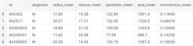
The dataset is taken from Kaggle and is part of the UCI Machine Learning repository. Columns are calculations made from a digitized image of a fine needle aspirate (FNA) exam of a breast mass. They describe the characteristics of the cell nuclei present in the image.

The computed values are:

a) radius (average of the distances from the center to the perimeter points)

b) texture (standard deviation of grayscale values)

c) perimeter

d) area

e) smoothness (local variation in ray lengths)

f) compaction (perimeter ^ 2 / area — 1.0)

g) concavity (severity of the concave portions of the contour)

h) concave points (number of concave portions of the contour)

i) symmetry

j) fractal dimension (“coastline approach” — 1)

We will start our project by importing the library Pandas, to read the data and perform a pre-processing.

import pandas as pd
df = pd.read_csv('../input/breast-cancer-wisconsin-data/data.csv')
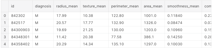
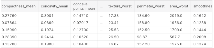
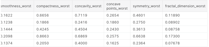
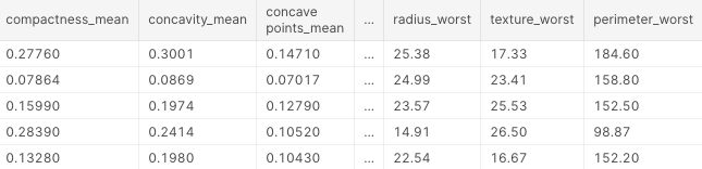
df.head()

These are the first 5 lines of our dataset:

Next, we’ll look for null values.

df.isnull().sum()

Of all columns, only one has:

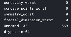
So we can delete it from our dataset. This is only possible because there are a lot of “lost” values in just one column. If it happened in others, we would have to carry out a different treatment to try to fill these gaps. Moving forward, we’ll delete the column and create a new DataFrame:

df_1 = df.drop(columns = "Unnamed: 32")
df_1.head()

Now, we can use a function called Label Encoder to “encode” our target variable, which we intend to use for diagnosis and transform its values into 0 and 1.

from sklearn.preprocessing import LabelEncoder
le = LabelEncoder()
df_1['diagnosis'] = le.fit_transform(df_1['diagnosis'])
df_1.head()

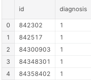
With this, we have that the benign will be 0 and the malignant 1. The confusion matrix below indicates the performance metrics of our algorithm, crossing the predicted results with the original observed classes.

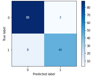
This matrix of confusion tells us that our algorithm got 88 True Positives right (in our case, malignant), 8 False Positives (predicted malignant, but they are benign), 3 False Negatives (predicted benign, but they are malignant) and 44 True Negatives (benign). This is the performance metric of our algorithm, described below.

After completing our initial pre-processing and analysis, we will move on to the Machine Learning algorithm.

The chosen one was the SVM. We will use train test split, a method of dividing arrays or matrices into training sets and random test subsets .

from sklearn.model_selection import train_test_split
from numpy import random

SEED = 10
random.seed(SEED)
treino_x, teste_x, treino_y, teste_y = train_test_split(exams, diagnosis)

We separate our dataset into training and test data, the x indicates the columns of the exam characteristics, while the y is our target value, that is, the diagnosis.

With that, the algorithm will “adapt” to this data and make the prediction.

from sklearn import svm
clf_1 = svm.SVC()
clf_1.fit(treino_x, treino_y)
acc_1 = clf_1.score(teste_x, teste_y)*100
print(" %.2f%%" % acc_1)

The accuracy of this model is:

Thank you for coming this far, I hope you enjoyed it!

Github: https://bit.ly/3oKANuv

Portfólio: https://bit.ly/3vh4PIO